Objectives

The learning objectives for this practical are:

Writing R scripts.
How to manipulate dates in data.
How to create and use factor objects.

Setup and background

To do this practical you need an installation of R and RStudio. You can find the instructions in the setup link on how to install R and RStudio in your system. For a smooth development of this practical, it is strongly recommended that you follow and finish the previous seminar 4 on how to get started with R and RStudio.

We will use the data files called mostres_analitzades.csv and virus_detectats.csv that were generated in the first practical. If you don’t have these files, please review that practical and generate them again. Once you have obtained those two files, copy them into a fresh new directory called practical7. The values obtained below have been obtained with the following specific versions (Feb 9, 2026) of these files:

Writing R scripts

We may often use an interactive R session to quickly examine data or make some straightforward calculations. In such an interactive session, we can also recover previous instructions in the R shell by pressing the upwards arrow key. However, if we really want to keep track of the R commands we are using, we should write them in a text file with filename extension .R, which we shall refer hereafter as an R script.

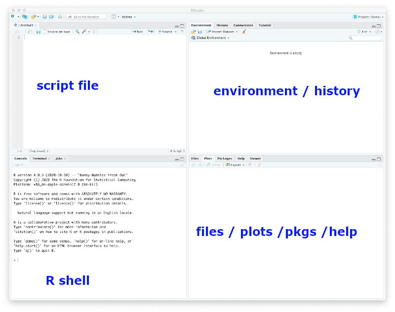
There are two main ways to create an R script: (1) opening a new file with a text editor and saving it with filename that includes the .R extension, or (2) if we are working with RStudio, then we click on the File menu and select the options New File -> R Script. When we do that we should be getting the RStudio window splitted in four panes, the default three ones and one additional one for the newly created R script, as shown in the captured window below.

Type in the newly created R script (either with a text editor or with RStudio) the following two lines to read the CSV file downloaded in the previous section. The first line is a comment. Lines starting with the # symbol are comments in R.

> ## read SIVIC data
> dat <- read.csv("mostres_analitzades.csv", stringsAsFactors=TRUE)

Now save the R script in the directory practical7 under the filename sivicanalysis.R.

To execute a specific line of an R script in RStudio you should move the cursor to that line in the pane with the script file and press the key combination Ctrl+Enter (Cmd+Enter in Apple computers). Alternatively, you can also copy and paste the line from the script to the R shell, specially if you are not working with RStudio.

The previous line may produce an error if the current working directory of R is not pointing to the directory where the file .csv is; see previous seminar 4 if you need to find out how to change the working directory in R and RStudio.

In general, changing the working directory should be always performed in the R shell and NEVER include the instruction that changes the working directory in an R script. The reason is because you or somebody else may want to run that script in a different computer where the directory with the data may be called differently.

You can examine the first 6 rows of the loaded CSV file with the head() function as follows:

> head(dat)

  setmana_epidemiologica  any data_inici data_final codi_regio
1                     12 2023 20/03/2023 26/03/2023         62
2                     44 2023 30/10/2023 05/11/2023         62
3                     32 2022 08/08/2022 14/08/2022         75
4                     27 2023 03/07/2023 09/07/2023         70
5                     42 2022 17/10/2022 23/10/2022         64
6                     11 2023 13/03/2023 19/03/2023         70
                    nom_regio codi_ambit                   nom_ambit sexe
1           Camp de Tarragona         62           Camp de Tarragona Dona
2           Camp de Tarragona         62           Camp de Tarragona Home
3 Barcelona Metropolitana Sud         75 Barcelona Metropolitana Sud Home
4                     Penedès         70                     Penedès Home
5                      Girona         64                      Girona Dona
6                     Penedès         70                     Penedès Home
  grup_edat index_socioeconomic total positiu
1   30 a 34                   2     1       1
2   30 a 34                   3     1       0
3   35 a 39                   2     1       1
4   60 a 64                   4     1       0
5   70 a 74                   3     1       1
6   70 a 74                   4     1       1

Exercise: tabulate the values of the column sexe with the function table(). Add to the script sivicanalysis.R the following two lines to obtain a new data.frame object called dat2 that excludes rows where the value in the column sexe is No disponible. You have to figure out the code that replaces the questions marks ?????? below.

> mask <- ??????
  dat2 <- dat[mask, ]

Once you subset data, it is always convenient to compare the dimensions of the original and resulting object, using the function dim(), and think whether the difference in dimensions makes sense (e.g., subsetting should always lead to a smaller object in some dimension), and whether the number of rows in this case matches the number of TRUE values in the logical mask.

Date-data management

These data have two columns called data_inici and data_final that corresponding to the begining and end of the 7-day period of the data of that row, but which are stored as string character vectors (more specifically as factors). However, R provides a way to store dates as such and this has the advantage that facilitates manipulating them for analysis purposes.

For instance, to transform the two columns containing date data we should use the function as.Date() as follows:

> startdate <- as.Date(dat2$data_inici, "%d/%m/%Y")
> enddate <- as.Date(dat2$data_final, "%d/%m/%Y")

Here the second argument informs the function as.Date() about the format of the input dates, in this case, day/month/4-digit-year corresponding to the format string "%d/%m/%Y. The help page of as.Date() contains full details about this. While R displays these objects as vectors of character strings in the format 4-digit-year-month-day, they do belong to a different class of objects, the class Date.

> head(startdate)

[1] "2023-03-20" "2023-10-30" "2022-08-08" "2023-07-03" "2022-10-17"
[6] "2023-03-13"

> class(startdate)

[1] "Date"

> head(enddate)

[1] "2023-03-26" "2023-11-05" "2022-08-14" "2023-07-09" "2022-10-23"
[6] "2023-03-19"

> class(enddate)

[1] "Date"

Having dates stored as Date-class objects facilitates operations on dates such as calculating time differences:

Calculating time differences:

> head(enddate - startdate + 1)

Time differences in days
[1] 7 7 7 7 7 7

Caculating earliest and latest time with the min() and max() functions:

> min(startdate)

[1] "2022-05-09"

> max(startdate)

[1] "2026-01-26"

Subsetting data for a period of time. For instance, let’s subset the data, selecting rows corresponding to the last academic year from September 2023 to June 2024:
```
> mask <- startdate >= as.Date("2023-09-01") & enddate <= as.Date("2024-06-30")
> sum(mask)

[1] 8079

> dat2yr2324 <- dat2[mask, ]
> dim(dat2yr2324)

[1] 8079   13
```
Note that the number of TRUE values in the logical mask matches the resulting number of rows in the subsetted object dat2yr2324.

Date data also allows one to easily extract the month of each date. Let’s extract again the starting date this time for the subsetted data, and see how do we get the months from those dates:

> startdate <- as.Date(dat2yr2324$data_inici, "%d/%m/%Y")
> m <- months(startdate, abbreviate=TRUE)
> head(m)

[1] "Oct" "Sep" "Oct" "Sep" "Oct" "Oct"

> class(m)

[1] "character"

where we have to use the argument abbreviate=TRUE in the months() function to obtain a vector of equally sized character strings, which may be useful for visualization purposes.

Important: The previous vector m may contain the names of the months in a different language than English when the regional configuration of your operating system, known as locale configuration, is also different to English. In such a case, it may be handy to switch at least the regional time configuration to English, to facilitate following the rest of this practical. To do that, type the following instruction on the R shell:

> Sys.setlocale("LC_TIME", "C")

and then type again:

> m <- months(startdate, abbreviate=TRUE)

Verify that now the vector m has the month names in English.

Factors

Factors in R are a class of objects that serve the purpose of storing what is known in statistics as a categorical variable, which is a variable that takes values from a limited number of categories, also known as levels. So factors are pretty much like vectors of character strings, but with additional information about what are the different values that may occur on those vectors.

Not all vectors of character strings are suitable to become factors. For instance, a vector of character strings corresponding to gene identifiers tipically should not become a factor in R, because those identifiers do not represent any kind of category grouping observations.

Factors are useful, however, in the context of a statistical analysis and data visualization, involving categorical variables. To create a factor object we should call the function factor() giving a vector of character strings as argument. Let’s consider converting the previous vector m of character strings to a factor.

> mf <- factor(m)
> head(mf)

[1] Oct Sep Oct Sep Oct Oct
Levels: Apr Dec Feb Jan Jun Mar May Nov Oct Sep

We can see that R displays factors differently to character strings, by showing the values without double quotes (") and providing additional information about the possible levels of that factor. We can access the level information from a factor object with the functions levels() and nlevels().

> levels(mf)

 [1] "Apr" "Dec" "Feb" "Jan" "Jun" "Mar" "May" "Nov" "Oct" "Sep"

> nlevels(mf)

[1] 10

Note that we have 10 levels instead of 12, because the subsetted data includes only the months corresponding to the academic year, i.e., from September to June.

Sometimes, we may want the levels of a factor to comprise a set of specific values or to be ordered in a specific way. This could be the case of the previous factor mf, where we would like for instance to have the levels corresponding to the months of the year and chronologically ordered. We can do that as follows:

> mf <- factor(m, levels=c("Jan", "Feb", "Mar", "Apr", "May", "Jun",
                           "Jul", "Aug", "Sep", "Oct", "Nov", "Dec"))
> head(mf)

[1] Oct Sep Oct Sep Oct Oct
Levels: Jan Feb Mar Apr May Jun Jul Aug Sep Oct Nov Dec

> levels(mf)

 [1] "Jan" "Feb" "Mar" "Apr" "May" "Jun" "Jul" "Aug" "Sep" "Oct" "Nov" "Dec"

> nlevels(mf)

[1] 12

Important: The previous call to the factor() function will only work if your regional time configuration is English. If you are working with a non-English regional time configuration, you should change the level names in the argument levels to the language that you are using.

Now, we can build a contingency table of the level occurrences of a factor using the function table().

> table(mf)

mf
 Jan  Feb  Mar  Apr  May  Jun  Jul  Aug  Sep  Oct  Nov  Dec 
1012  860  872  905  739  672    0    0  648  980  812  579

We can see, there is no data for the months of July and August. We can remove levels of a factor for which there is no data with the function droplevels().

> mf <- droplevels(mf)
> levels(mf)

 [1] "Jan" "Feb" "Mar" "Apr" "May" "Jun" "Sep" "Oct" "Nov" "Dec"

> table(mf)

mf
 Jan  Feb  Mar  Apr  May  Jun  Sep  Oct  Nov  Dec 
1012  860  872  905  739  672  648  980  812  579

One of the common uses of a factor is to aggregate numerical values by the levels of that factor. For instance, in our previous data, the column positiu contains the number of positively tested individuals, but each value in that column corresponds to the number per week, region, sex, age group and socioeconomical index. Let’s say we want to aggregate those positively tested individuals per month in the data.frame object dat2yr2324. We can use the function aggregate() for that purpose, as follows:

> posbymonth <- aggregate(dat2yr2324$positiu, list(month=mf), sum)

Here the first argument is the vector (column of dat2yr2324 in this case) with numerical values that we want to aggregate, the second argument is a list object with one element for each factor whose levels we want to use to group the values, and the third argument is the function we want to use to summarize the data per group. The result is a data.frame object with one column per factor and a final column called x with the aggregate values:

> posbymonth

   month   x
1    Jan 992
2    Feb 721
3    Mar 752
4    Apr 690
5    May 560
6    Jun 554
7    Sep 495
8    Oct 778
9    Nov 770
10   Dec 543

We can visualize these data in a scatter plot by converting the factor into an integer, and plotting the month into the x-axis and the numerical value into the y-axis:

> plot(as.integer(posbymonth$month), posbymonth$x, type="b")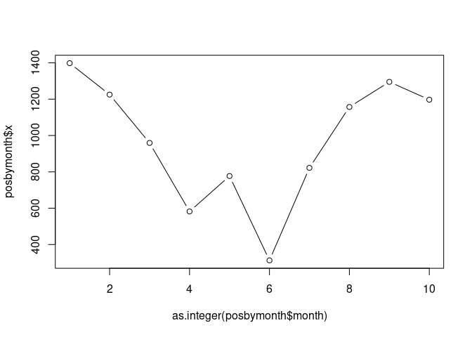

Exercise: look up in the help page of the plot() function, how can you change the labels for the x and y axes to a readable label whose meaning stands alone and minimally describes the data visualized in that axis. The resulting plot should be identical to the one above, but with the axes labels changed.

Exercise: Repeat the same plot, but instead of aggregating the number of positive cases, aggregate the positive rate by first calculating it using the columns total and positiu, and then using the mean() function to aggregate the values. Can you interpret the resulting plot?

Exercise: Aggregate again the positive rate as in the previous exercise, but this time by two factors, month and age group (look up in the data.frame object dat2yr2324 which column may store the age group). Assuming the result of the function aggregate() is stored into a data.frame object called posrbymonthage, plot the aggregated positive rate as function of the month using the following plotting instruction:

> plot(posrbymonthage$x ~ posrbymonthage$month,
       xlab="Month", ylab="Positive rate")

The resulting plot contains so-called box plots for each month, which allow one to visualize the location and spread of the data in terms of quartiles. How would you interpret the different sizes of the boxes throughout the months of the year?